Today’s blog post is an article and coding demonstration that details conjoint analysis in R and how it’s useful in marketing data science.

What is conjoint analysis? And how can it be used in marketing data science?

Conjoint analysis is one of the most widely-used quantitative methods in marketing research and analytics.  It gets under the skin of how people make decisions and what they really value in their products and services.

Conjoint analysis can be quite important, as it is used to:

• Measure the preferences for product features
• See how changes in pricing affect demand for products or services
• Predict the rate at which a product is accepted in the market

Conjoint analysis in R can help businesses in many ways. Want to understand if the customer values quality more than price? Conjoint analysis has you covered! Do you want to know whether the customer consider quick delivery to be the most important factor? We can tell you! Conjoint analysis in R can help you answer a wide variety of questions like these.

The usefulness of conjoint analysis is not limited to just product industries. Even service companies value how this method can be helpful in determining which customers prefer the most – good service, low wait time, or low pricing.

For businesses, understanding precisely how customers value different elements of the product or service means that product or service deployment can be much easier and can be optimized to a much greater extent. Identifying key customer segments helps businesses in targeting the right segments. A good example of this is Samsung.

Samsung produces both high-end (expensive) phones along with much cheaper variants. Behind this array of offerings, the company is segmenting its customer base into clear buckets and targeting them effectively. Conjoint analysis is used quite often for segmenting a customer base.

Let’s look at a few more places where conjoint analysis is useful.

• Predicting what the market share of a proposed new product or service might be considering the current alternatives in the market
• Understanding consumers’ willingness to pay for a proposed new product or service
• Quantifying the tradeoffs customers are willing to make among the various attributes or features of the proposed product/service

Alright, now that we know what conjoint analysis is and how it’s helpful in marketing data science, let’s look at how conjoint analysis in R works.

Coding up a conjoint analysis in R

Let’s start with an example. Using the smartphone as an example, imagine that you are a product manager in a company which is ready to launch a new smartphone. Now, instead of surveying each individual customer to determine what they want in their smartphone, you could use conjoint analysis in R to create profiles of each product and then ask your customers or potential customers how they’d rate each product profile. Maybe you get something like this…

The columns are profile attributes and the rows are “levels”. Each row represents its own product profile. There are 3 product profiles in the above table. You can use ordinary least square regression to calculate the utility value for each level.  Below is the equation for the same.

Y = β0 + β1X +… βzXzϵ

Now let’s start with carrying out conjoint analysis in R.

> library(conjoint)
> ## Loading in the data
> data(tea)

The tea data set contains survey response data for 100 people on what sort of tea would they prefer to drink.

> str(tprof)
'data.frame':	13 obs. of  4 variables:
 $ price  : int  3 1 2 2 3 2 3 2 3 1 ...
 $ variety: int  1 2 2 1 3 1 2 3 1 3 ...
 $ kind   : int  1 1 2 3 3 1 1 1 2 2 ...
 $ aroma  : int  1 1 1 1 1 2 2 2 2 2 ...

You can see that there are four attributes, namely:
1. Price
2. Variety
3. Kind
4. Aroma

Let’s look at the survey data. There are 100 observations with 13 profiles.

> str(tprefm)
'data.frame':	100 obs. of  13 variables:
 $ profil1 : int  8 0 4 6 5 10 8 5 7 8 ...
 $ profil2 : int  1 10 10 7 1 1 0 2 3 7 ...
 $ profil3 : int  1 3 3 4 7 1 0 1 3 3 ...
 $ profil4 : int  3 5 5 9 8 5 0 4 9 10 ...
 $ profil5 : int  9 1 4 6 6 1 9 3 0 9 ...
 $ profil6 : int  2 4 1 3 10 0 0 8 5 1 ...
 $ profil7 : int  7 8 2 7 7 0 0 5 3 2 ...
 $ profil8 : int  2 6 0 4 10 0 0 9 0 2 ...
 $ profil9 : int  2 2 0 8 6 0 0 6 5 2 ...
 $ profil10: int  2 9 1 5 6 0 0 8 0 2 ...
 $ profil11: int  2 7 8 2 6 0 5 3 5 8 ...
 $ profil12: int  3 5 9 10 10 1 10 1 10 10 ...
 $ profil13: int  4 2 7 9 7 1 8 2 8 8 ...

The different levels are:

> tlevn
       levels
1         low
2      medium
3        high
4       black
5       green
6         red
7        bags
8  granulated
9       leafy
10        yes
11         no

Now let’s calculate the utility value for just the first customer.

> caModel(y=tprefm[1,], x=tprof)

Call:
lm(formula = frml)

Residuals:
      1       2       3       4       5       6       7       8 
 1.1345 -1.4897  0.3103 -0.2655  0.3103  0.1931  1.5931 -1.4310 
      9      10      11      12      13 
-1.4310  1.1207  0.3690  1.1931 -1.6069 

Coefficients:
                   Estimate Std. Error t value Pr(>|t|)   
(Intercept)          3.3937     0.5439   6.240  0.00155 **
factor(x$price)1    -1.5172     0.7944  -1.910  0.11440   
factor(x$price)2    -1.1414     0.6889  -1.657  0.15844   
factor(x$variety)1  -0.4747     0.6889  -0.689  0.52141   
factor(x$variety)2  -0.6747     0.6889  -0.979  0.37234   
factor(x$kind)1      0.6586     0.6889   0.956  0.38293   
factor(x$kind)2     -1.5172     0.7944  -1.910  0.11440   
factor(x$aroma)1     0.6293     0.5093   1.236  0.27150   
---
Signif. codes:  0 ‘***’ 0.001 ‘**’ 0.01 ‘*’ 0.05 ‘.’ 0.1 ‘ ’ 1

Residual standard error: 1.78 on 5 degrees of freedom
Multiple R-squared:  0.8184,	Adjusted R-squared:  0.5642 
F-statistic:  3.22 on 7 and 5 DF,  p-value: 0.1082

> caUtilities(y=tprefm[1,], x=tprof, z=tlevn)

Call:
lm(formula = frml)

Residuals:
      1       2       3       4       5       6       7       8 
 1,1345 -1,4897  0,3103 -0,2655  0,3103  0,1931  1,5931 -1,4310 
      9      10      11      12      13 
-1,4310  1,1207  0,3690  1,1931 -1,6069 

Coefficients:
                   Estimate Std. Error t value Pr(>|t|)   
(Intercept)          3,3937     0,5439   6,240  0,00155 **
factor(x$price)1    -1,5172     0,7944  -1,910  0,11440   
factor(x$price)2    -1,1414     0,6889  -1,657  0,15844   
factor(x$variety)1  -0,4747     0,6889  -0,689  0,52141   
factor(x$variety)2  -0,6747     0,6889  -0,979  0,37234   
factor(x$kind)1      0,6586     0,6889   0,956  0,38293   
factor(x$kind)2     -1,5172     0,7944  -1,910  0,11440   
factor(x$aroma)1     0,6293     0,5093   1,236  0,27150   
---
Signif. codes:  0 ‘***’ 0,001 ‘**’ 0,01 ‘*’ 0,05 ‘.’ 0,1 ‘ ’ 1

Residual standard error: 1,78 on 5 degrees of freedom
Multiple R-squared:  0,8184,	Adjusted R-squared:  0,5642 
F-statistic:  3,22 on 7 and 5 DF,  p-value: 0,1082

 [1]  3.3936782 -1.5172414 -1.1413793  2.6586207 -0.4747126
 [6] -0.6747126  1.1494253  0.6586207 -1.5172414  0.8586207
[11]  0.6293103 -0.6293103

The higher the utility value, the more importance that the customer places on that attribute’s level.

The estimate from the Ordinary Least Squares model gives the utility values for this first customer. The higher the utility value, the more importance that the customer places on that attribute’s level.

Let’s look at the utility values for the first 10 customers. You can do this by:

> caPartUtilities(y=tprefm[1:10,], x=tprof, z=tlevn)
      intercept    low medium   high  black  green    red   bags
 [1,]     3.394 -1.517 -1.141  2.659 -0.475 -0.675  1.149  0.659
 [2,]     5.049  3.391 -0.695 -2.695 -1.029  0.971  0.057  1.105
 [3,]     4.029  2.563 -1.182 -1.382 -0.248  2.352 -2.103 -0.382
 [4,]     5.856 -1.149 -0.025  1.175 -0.492  1.308 -0.816 -0.825
 [5,]     6.250 -2.333  2.567 -0.233 -0.033 -0.633  0.667 -0.233
 [6,]     1.578 -0.713 -0.144  0.856  1.456 -0.744 -0.713  0.656
 [7,]     2.635 -0.920 -1.040  1.960 -0.707  0.293  0.414 -1.107
 [8,]     4.405 -0.425  0.413  0.013  0.546 -2.454  1.908  1.479
 [9,]     3.546 -0.966  0.883  0.083  2.216  1.416 -3.632 -0.917
[10,]     5.460  0.678 -0.639 -0.039  0.228  0.428 -0.655 -1.172
      granulated  leafy    yes     no
 [1,]     -1.517  0.859  0.629 -0.629
 [2,]     -0.609 -0.495 -0.681  0.681
 [3,]     -2.437  2.818  0.776 -0.776
 [4,]     -0.149  0.975  0.121 -0.121
 [5,]     -0.333  0.567 -1.250  1.250
 [6,]     -0.713  0.056  1.595 -1.595
 [7,]     -2.586  3.693  0.147 -0.147
 [8,]      0.241 -1.721 -1.060  1.060
 [9,]     -0.966  1.883 -0.259  0.259
[10,]     -2.655  3.828  1.414 -1.414

To understand the requirement of the surveyed population as a whole, let’s run the test for all the respondents.

> Conjoint(y=tpref, x=tprof, z=tlevn)

Call:
lm(formula = frml)

Residuals:
    Min      1Q  Median      3Q     Max 
-5,1888 -2,3761 -0,7512  2,2128  7,5134 

Coefficients:
                   Estimate Std. Error t value Pr(>|t|)    
(Intercept)         3,55336    0,09068  39,184  < 2e-16 ***
factor(x$price)1    0,24023    0,13245   1,814    0,070 .  
factor(x$price)2   -0,14311    0,11485  -1,246    0,213    
factor(x$variety)1  0,61489    0,11485   5,354 1,02e-07 ***
factor(x$variety)2  0,03489    0,11485   0,304    0,761    
factor(x$kind)1     0,13689    0,11485   1,192    0,234    
factor(x$kind)2    -0,88977    0,13245  -6,718 2,76e-11 ***
factor(x$aroma)1    0,41078    0,08492   4,837 1,48e-06 ***
---
Signif. codes:  0 ‘***’ 0,001 ‘**’ 0,01 ‘*’ 0,05 ‘.’ 0,1 ‘ ’ 1

Residual standard error: 2,967 on 1292 degrees of freedom
Multiple R-squared:  0,09003,	Adjusted R-squared:  0,0851 
F-statistic: 18,26 on 7 and 1292 DF,  p-value: < 2,2e-16

[1] "Part worths (utilities) of levels (model parameters for whole sample):"
       levnms    utls
1   intercept  3,5534
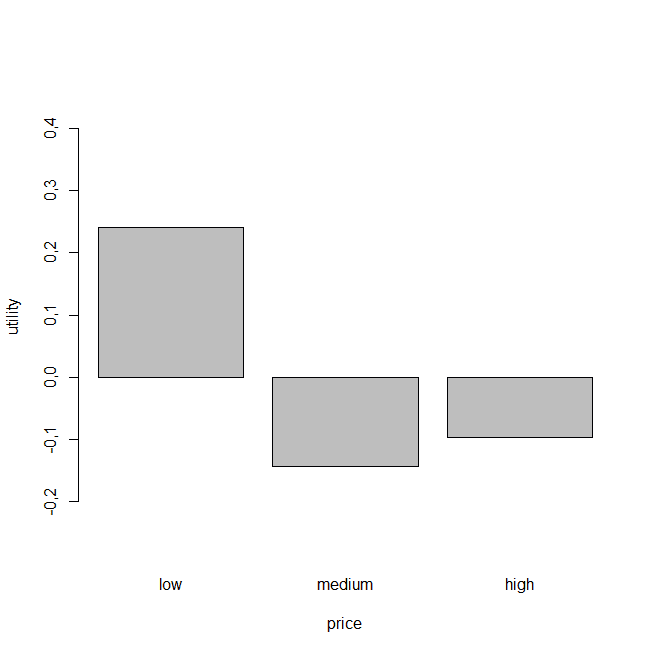
2         low  0,2402
3      medium -0,1431
4        high -0,0971
5       black  0,6149
6       green  0,0349
7         red -0,6498
8        bags  0,1369
9  granulated -0,8898
10      leafy  0,7529
11        yes  0,4108
12         no -0,4108
[1] "Average importance of factors (attributes):"
[1] 24,76 32,22 27,15 15,88
[1] Sum of average importance:  100,01
[1] "Chart of average factors importance"

Data above shows the utility scores for the whole population. Let’s also look at some graphs so we can easily understand the utility values.

Numerically, the attribute values are as follows:

1. Price: 24.76
2. Variety: 32.22
3. Kind: 27.15
4. Aroma: 15.88

This plot tells us what attribute has most importance for the customer – Variety is the most important factor.

Now let’s look at the individual level utilities for each attribute:

We already know that variety is the most important consideration for the customers, but now we can also see from the graph (above) that the “black” variety has the highest utility score. What this means is that – although product variety is the most important factor about the tea selection, customers prefer the black tea above all others.

Now that we’ve completed the conjoint analysis, let’s segment the customers into 3 or more segments using the k-means clustering method.

> caSegmentation(y=tpref, x=tprof, c=3)
K-means clustering with 3 clusters of sizes 29, 31, 40

Cluster means:
      [,1]     [,2]     [,3]     [,4]     [,5]     [,6]     [,7]
1 4.808000 5.070759 2.767310 7.132138 6.843172 2.649483 3.656379
2 3.330226 5.582000 5.214258 4.207645 3.859419 4.740871 5.173129
3 5.480275 2.938100 1.368100 4.540275 1.973100 3.782900 1.382900
      [,8]     [,9]    [,10]    [,11]    [,12]    [,13]
1 1.539724 2.063862 1.030862 6.691448 5.980517 6.801207
2 5.334710 3.366968 4.838194 4.612129 6.050548 5.108613
3 0.965750 2.820750 0.111225 3.450750 0.442900 0.692900

Clustering vector:
  [1] 1 2 1 2 2 3 1 2 1 1 1 1 3 3 3 3 2 3 2 3 3 1 3 2 2 1 2 2 2 2 3
 [32] 1 2 1 1 1 1 3 3 3 3 2 3 2 3 1 1 3 3 3 1 3 3 3 2 1 3 2 3 2 3 3
 [63] 1 2 2 1 3 3 3 2 1 3 1 2 1 2 2 3 1 1 2 2 2 1 3 3 3 3 2 3 2 3 2
 [94] 3 3 1 3 2 1 1

The clustering vector shown above contains the cluster values. Let’s visualize these segments.

Now we’ve broken the customer base down into 3 groups, based on similarities between the importance they placed on each of the product profile attributes.